[POSTECH Industry–Academia Research] Vehicle Speed Estimation from Low-FPS CCTV


[EVA × POSTECH Industry–Academia Collaboration] This research was conducted by Jaehun Hwang and Keonwoo Park of the POSTECH AIM Lab under the supervision of Professor Minseok Song.
Introduction: From Object Detection to Motion Understanding
Detecting a vehicle in a video is not enough to determine whether it is speeding or approaching a hazardous area. To estimate its speed in km/h, the system must connect observations of the same vehicle over time and convert its movement in the image into a real-world distance.
The goal of this research was to maintain stable vehicle identities in low-FPS CCTV footage, calibrate the camera view against real-world road coordinates, and generate speed information that EVA can use.
Rather than simply replacing a tracking model, the research team implemented and validated the entire pipeline—from associating vehicles at low frame rates to converting pixel coordinates into real-world distances and presenting speed results in a verification interface. The demo below shows vehicle IDs, trajectories, a measurement area, and estimated speeds together.
Vehicle speed estimation running in EVA
1. Image Feature Extraction: Describing Vehicle Appearance
In low-FPS footage, a vehicle may travel far enough between frames that its previous and current bounding boxes no longer overlap. Because position alone is insufficient to identify the same vehicle, each detected vehicle crop is converted into a feature vector that can be compared over time.
Why did we need three features?
The visual cues that distinguish vehicles can be divided into shape, color, and contour. Each cue was reliable under different conditions, which made it difficult for a single feature to handle every CCTV environment consistently.
| Feature | Strength | Limitation |
|---|---|---|
| DINOv2 | Captures vehicle type, body shape, and general visual appearance | Fine-grained differences may weaken in low-resolution footage or between similar vehicles |
| HSV | Quickly separates vehicles of the same type when their body colors differ | Sensitive to shadows, backlighting, nighttime illumination, and exposure changes |
| HOG | Uses contours and intensity gradients when color information is weak | Contours change under rotation, occlusion, and truncated bounding boxes |
DINOv2: Representing Overall Vehicle Appearance
DINOv2 extracts a deep feature that combines shape, texture, and visual components. Early in the research, we also evaluated Qwen visual features because they aligned naturally with EVA's VLM direction. VLMs are strong at semantic similarity, however, while tracking must distinguish individual vehicles that may look almost identical. When we compared the score distributions for matching and non-matching vehicles, DINOv2 separated the two groups more clearly, so we selected it as the default deep feature model.
HSV: Quantifying Color Distribution
HSV separates hue, saturation, and value. After converting a vehicle crop from RGB to HSV, we accumulate H, S, and V values in predefined histogram bins to create a feature vector that represents which colors, and how much of each color, appear on the vehicle.
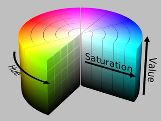

The HSV color space (left) and an example of accumulating pixel values by histogram bin (right)
We compare two vehicles' color distributions with histogram intersection, which sums the smaller value in each corresponding bin. Greater overlap produces a higher score, helping separate vehicles with similar types but different body colors.
HOG: Quantifying Contours and Intensity Boundaries
HOG converts each vehicle crop to grayscale, then calculates the direction and magnitude of brightness changes at every pixel. It builds a histogram of gradient directions within small cells, normalizes neighboring cells together as blocks, and concatenates the results into a contour feature that relies less on color.
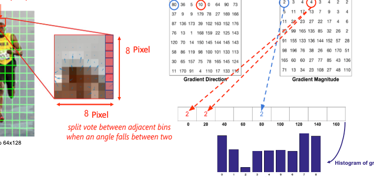
HOG represents the direction and strength of brightness changes as a directional histogram
Source: LearnOpenCV
No single feature was sufficient for every scene. HSV was especially effective when daytime color information was clear, while HOG contours provided a useful fallback when color cues weakened. We therefore normalized and fused the three scores using a baseline ratio of DINOv2 0.3 : HSV 0.5 : HOG 0.2.
This fusion allows the remaining features to support a match when one signal is disrupted by lighting or occlusion. Although the ideal weights can vary by scene, using all three provided a stable common baseline across different CCTV environments. The fused representation acts as a visual fingerprint for comparing past tracks with current detections.
2. Low-FPS Tracking: Linking IDs with Appearance and Motion
Connecting vehicles based only on similar image features can swap their IDs when vehicles of the same color and type appear together. Motion alone also fails when a vehicle has just entered the scene or when the interval between frames is long. We therefore designed the tracker to use appearance as its primary matching signal and motion as supporting evidence.
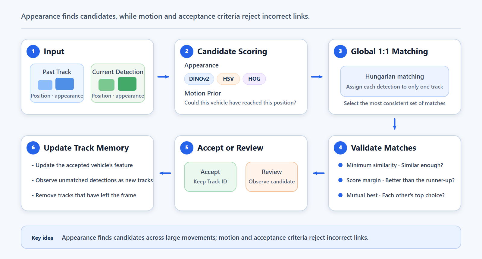
Feature similarities are fused, and only candidates that pass motion and score gates are linked one-to-one
First, the tracker calculates fused-feature similarity for every combination of past track and current detection. For tracks with enough history, it adds a motion prior based on recent direction and speed to check whether the vehicle could plausibly have reached the observed position. Appearance finds candidates across large movements; motion checks whether each candidate is physically plausible.
Hungarian matching then assigns candidates globally without duplicates. An assignment is not accepted automatically. The tracker checks whether the similarity is high enough, whether it is clearly better than the next candidate, and whether the track and detection rank each other first.
If a pair fails those checks, the tracker removes that combination and searches the remaining candidates again. This recovers valid alternatives hidden by the first assignment without forcing an uncertain link. Only accepted observations update track memory, while new detections and tracks that have left the scene are managed separately to keep a single false detection from contaminating later matches.
Improving Tracking Performance at Night
At night, both color and position cues become less reliable. Emergency lights and headlights can sharply change the HSV distribution of the same vehicle from one frame to the next. A detection box may also follow glare or a road reflection instead of the vehicle body, making the vehicle appear to move against its true direction. Because the next observation is already far away at low frame rates, neither appearance nor motion alone can reliably recover from this error.

Frames shown in chronological order. As the bounding box follows a glare blob, the observed ground-contact point moves opposite to the vehicle's direction of travel
Rather than relaxing every threshold, we adjusted the feature combination, candidate comparison, and track-retention policy for the causes of nighttime failure.
| Change | Nighttime configuration | Intended effect |
|---|---|---|
| Candidate competition | Excludes candidates already assigned to another pair from margin and mutual-best competition | Prevents a correct match from being rejected because of a candidate that can no longer be assigned |
| Fusion | Removes HSV from weights, thresholds, and absolute floors; uses DINOv2 0.8 : HOG 0.2 | Limits the effect of abrupt HSV changes while glare appears or clears |
| Track lifecycle | Reduces lost-track retention from five frames to three | Prevents stale tracks from continuing to distort normalization and competition scores |
| New tracks | Lowers the detection-confidence threshold from 0.5 to 0.4, but issues a new ID only when track confidence is at least 0.6 | Reduces nighttime missed detections while suppressing unnecessary IDs from false positives and partial detections |
At 1 FPS on 12 UA-DETRAC sequences, these changes raised IDF1 from 64.0 to 75.3 and MOTA from 56.5 to 64.8, while reducing ID switches from 640 to 176. Replacing the deep feature accounted for about 15% of the improvement; the remainder came from the revised competition rules and nighttime-specific gates and lifecycle. The result reinforced that good features alone are not enough: the tracker also needs a consistent policy for when to reject and when to revisit uncertain associations.
3. Camera Calibration: Converting Pixels into Meters
Tracking provides the pixel position of a vehicle and the time of each observation. Perspective, however, means that the same pixel displacement represents different real-world distances near and far from the camera. Pixel coordinates must therefore be projected onto a road plane measured in meters before speed can be calculated.
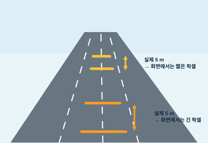
Perspective example: the same real-world distance of 5 m appears as different pixel lengths
The speed-estimation flow is straightforward.
Tracking first connects positions and capture times for the same vehicle, while calibration projects the vehicle's position from the image onto the road plane in meters. Finally, the system compares the real-world distance traveled with the elapsed time to estimate speed.
We initially investigated automatic calibration using monocular depth, an assumed average vehicle length, and vanishing points. Although convenient, this approach was sensitive to small estimation errors in CCTV scenes combining low frame rates, turning vehicles, and indistinct lane markings. It could also produce plausible but incorrect results whose cause was difficult for an operator to verify.
The final design therefore uses user-defined calibration. The user identifies reliable geometric references on the road plane, while the system calculates, validates, and stores the homography. It supports two input methods:
A homography unfolds the road area, which appears trapezoidal in the image, into a top-down plane. By matching image points with known road-plane coordinates, the system can convert vehicle positions from pixels into meters.
- Four corners and the real length and width of an area that is rectangular on the road plane
- At least four reference points with known real-world
(X, Y)coordinates, including points matched to a site plan
BrnoCompSpeed is a public benchmark dataset for vehicle-speed estimation that provides fixed-road-camera footage with ground-truth vehicle speeds.
Using actual tracking trajectories from nine of its camera views, we measured the following mean absolute errors.
| Calibration reference | Mean absolute error |
|---|---|
| Dataset ground-truth area | 1.13 km/h |
| Short rectangle | 7.48 km/h |
| Long rectangle aligned with travel direction | 1.52 km/h |
The resulting guideline is straightforward.
Place the calibration area where vehicles actually travel and make it as long as practical in the direction of travel. A one-meter input error creates a much larger relative error over a short area than over a long one. For projecting each vehicle onto the road plane, a single point at the bottom center of the bounding box was more stable than averaging multiple points.
4. Estimating Real-World Road Dimensions with a VLM
User-defined calibration requires the real length and width of the selected road area. Direct measurement remains the safest source, but an operator may not know the appropriate region or initial values when configuring a new camera. We therefore evaluated whether a VLM could inspect the marked road area and surrounding scene, then suggest initial real-world dimensions.
In the experiment, the four corners were labeled P1–P4, and the measurement area was emphasized with a blue outline and semi-transparent red fill. The most stable results came from providing both the annotated image and the four pixel coordinates while keeping the question concise. An image alone or coordinates alone performed less consistently.
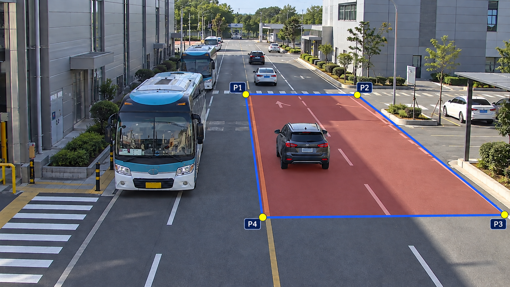
Example road-area overlay provided to the VLM
Using Qwen3.8-27B-FP8, we evaluated the improved input format on 21 images spanning three camera views across seven scenes.
Mean ratio error measures how far the VLM's estimated length and width deviate from the actual values on average; lower is better.
| Evaluation metric | Initial method | Final input method |
|---|---|---|
| Mean ratio error | 50.16% | 25.84% |
| Mean absolute length error | - | 7.80 m |
| Mean absolute width error | - | 1.83 m |
| Both dimensions within 10 m | - | 18/21 (85.7%) |
The revised input nearly halved the mean ratio error, but a 7.80-meter mean length error was still too large to use as the definitive metric scale for speed estimation. Longer perspective instructions and explicit reasoning did not improve every scene consistently.
At this stage, the VLM is therefore better suited as a configuration guide that a person can verify than as an automatic source of ground truth.
5. Speed Estimation Using Capture Timestamps
The final speed estimator uses three pieces of information together:
- The track ID links observations of the same vehicle.
- The calibration result converts the bottom center of the bounding box into metric road coordinates.
- The actual capture time provides the elapsed time instead of relying on frame count.
The estimator maintains a short position history for each track, then checks how far apart the first and last points in the recent window are on the road plane. It calculates average speed by comparing that real-world distance with the actual capture-time difference.
Using capture timestamps preserves the correct time basis even when the input frame rate changes. An exponential moving average reduces small fluctuations caused by bounding-box jitter.
The current output is not an instantaneous speed. It is the average ground-plane speed between the endpoints of the recent window. Curved paths may therefore be underestimated, while camera shake and non-planar roads require additional handling.
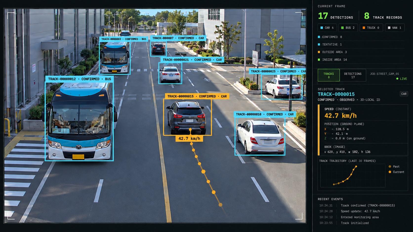
Vehicle speed estimation demo
6. Productization Roadmap: From Research to an EVA Feature
The purpose of this research was not limited to calculating vehicle speed. It was also intended to establish the foundation of an EVA feature that site operators can configure and use in practice. Combining vehicle speed and direction with EVA's detection zones, object information, and event rules enables the system to recognize scenarios such as the following.
| Scenario | Example application |
|---|---|
| Speeding detection | Alert when a vehicle exceeds the limit on factory roads, logistics sites, or campuses |
| Hazardous approach detection | Detect a vehicle rapidly approaching a worker, facility, or restricted area |
| Sudden acceleration or deceleration | Identify abnormal driving behavior involving a sharp speed change |
| Abnormally slow movement or congestion | Detect vehicles moving too slowly or remaining congested in a travel zone |
| Operational analytics | Show speed distributions and hazardous-event trends by time and zone in a dashboard |
This research was not limited to validating technical performance. It was conducted with productization in mind, considering the UX through which users configure the feature and verify its results. An operator can draw the vehicle measurement area directly on the camera view, receive initial length and width suggestions from the VLM, and confirm or correct them using site information or physical measurements. An overlay preview then displays the area, vehicle trajectories, and estimated speeds together so that the configuration can be checked immediately.
Once calibration is complete, users will be able to choose speed limits and target scenarios for each zone, then connect detected events to EVA alert channels and dashboards. A validated calibration can be reused for a fixed camera, while the interface can request recalibration after the camera position or zoom changes. The central UX goal is to hide unnecessary technical complexity while keeping the basis of the configuration and its results easy to verify.
The vehicle speed estimation technology developed through this research will go through productization—including site-specific setup guidance, VLM-assisted initial values, result-validation views, scenario configuration, and alert integration—and be released as an official EVA feature.